Multiprocessing in Python – all about pickling

Chances are you heard that multiprocessing in Python is hard. That it takes time and, actually, don’t even try because there’s something like global interpreter lock (GIL), so it isn’t even true parallel execution. Well, GIL is true, but the rest is a lie. Multiprocessing in Python is rather easy.

One doesn’t have to look far to find nice introductions into processing in Python [link1, link2]. These are great and I do recommend reading on them. Even first Google result page should return some comprehensible tutorials. However, what I was missing from these tutorials is some information about handling processing within class.

Multiprocessing in Python is flexible. You can either define Processes and orchestrate them as you wishes, or use one of excellent methods herding Pool of processes. By default Pool assumes number of processes to be equal to number of CPU cores, but you can change it by passing processes parameter. Main methods included in Pool are apply and map, which let you run process with arbitrary arguments or execute parallel map, respectively. There are also asynchronous versions of these, i.e. apply_asyncand map_async.

Quick example:

from multiprocessing import Pool
def power(x, n=10):
    return x**n

pool = Pool()
pow10 = pool.map(power, range(10,20))
print(pow10)
[10000000000, 25937424601, 61917364224, 137858491849, 289254654976, 576650390625, 1099511627776, 2015993900449, 3570467226624, 6131066257801]

Simple, right? Yes, this is all what’s needed. Now, go and use multiprocessing!

Actually, before you leave to follow your dreams there’s a small caveat to this. When executing processes Python first pickles these methods. This create a bottleneck as only objects that are pickle will be passed to processes. Moreover, Pool doesn’t allow to parallelize objects that refer to the instance of pool which runs them. It sounds convoluted so let me exemplify this:

from multiprocessing import Pool

class BigPow:
    def __init__(self, n=10):
        self.pool = Pool()

        self.n = n

    def pow(self, x):
        return x**self.n

    def run(self, args):
        #pows = self.pool.map(ext_pow, args)
        pows = self.pool.map(self.pow, args)
        return sum(pows)

def ext_pow(x):
    return x**10

if __name__ == "__main__":
    big_pow = BigPow(n=10)
    pow_sum = big_pow.run(range(20))
    print(pow_sum)

Code above doesn’t work, unless we replace self.pow with ext_pow. This is because self contains pool instance. We can remove that through removing pool just before pickling through __getstate__ (there’s complimentary function __setstate__ to process after depickling).

from multiprocessing import Pool

class BigPow:
    def __init__(self, n=10):
        self.pool = Pool()

        self.n = n

    def pow(self, x):
        return x**self.n

    def run(self, args):
        pows = self.pool.map(self.pow, args)
        return sum(pows)

    def __getstate__(self):
        self_dict = self.__dict__.copy()
        del self_dict['pool']
        return self_dict

if __name__ == "__main__":
    big_pow = BigPow(n=10)
    pow_sum = big_pow.run(range(20))
    print(pow_sum)

This is good, but sometimes you’ll get an error stating something like “PicklingError: Can’t pickle : attribute lookup __builtin__.instancemethod failed”. In such case you have to update registry for pickle on what to actually goes into pickling.

from multiprocessing import Pool

#######################################
import sys
import types
#Difference between Python3 and 2
if sys.version_info[0] < 3:
    import copy_reg as copyreg
else:
    import copyreg

def _pickle_method(m):
    class_self = m.im_class if m.im_self is None else m.im_self
    return getattr, (class_self, m.im_func.func_name)

copyreg.pickle(types.MethodType, _pickle_method)
#######################################

class BigPow:
    def __init__(self, n=10):
        self.pool = Pool()

        self.n = n

    def pow(self, x):
        return x**self.n

    def run(self, args):
        pows = self.pool.map(self.pow, args)
        return sum(pows)

    def __getstate__(self):
        self_dict = self.__dict__.copy()
        del self_dict['pool']
        return self_dict

if __name__ == "__main__":
    big_pow = BigPow(n=10)
    pow_sum = big_pow.run(range(20))
    print(pow_sum)

Yes, this is all because of Pickle. What can you do with it? In a sense, not much, as it’s the default battery-included solution. On the other, pickle is generally slow and now community standard seems to be dill. It would be nice if something was using dill instead of pickle. Right? Well, we are in luck because pathos does exactly that. It has similar interface to multiprocessing is it’s also easy to use. Personally I’m Ok with multiprocessing, as I like not to import too much, but this is a good sign that there are developments towards more flexible solutions.

Kuramoto in Stan (PyStan)

tl;dr: Project on github: https://github.com/laszukdawid/pystan-kuramoto


Stan is a programming language focused on probabilistic computations. Although it’s a rather recent language it’s been nicely received in data science/Bayesian community for its focus on designing model, rather than programming and getting stuck with computational details. Depending what is your background you might have heard about it either from Facebook and its Prophet project or as a native implementation for Hamiltonian Monte Carlo (HMC) and its optimised variation – No-U-Turn Sampler for HMC (NUTS).

For ease of including models in other programmes there are some interfaces/wrappers available, including RStan and PyStan.

Stan is not the easiest language to go through. Currently there are about 600 pages of documentation and then separate “documentations” for wrappers, which for PyStan isn’t very helpful. Obviously there’s no need for reading all of it, but it took me a while to actually understand what goes where an why. The reward, however, is very satisfying.

Since I’ve written a bit about Kuramoto models on this blog, it’s consistent if I share its implementation in Stan as well. Pystan-kuramoto project uses PyStan, but the actual Stan code is platform independent.

Currently there are two implementations (couldn’t come up with better names):

  • All-to-all, where Kuramoto model fit is performed to phase vector \vec{\Phi} 
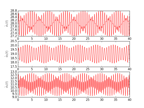
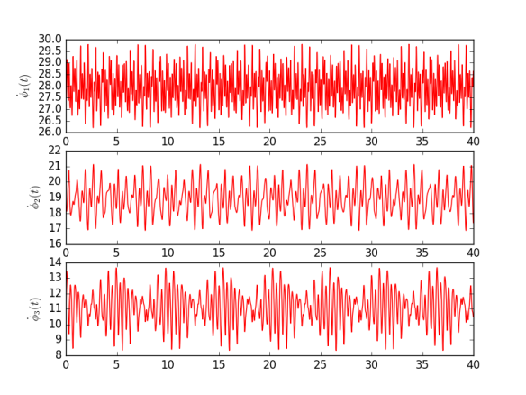
with distinct oscillators, i.e. \vec{\Phi}_{N}(t) = \{\phi_1(t), \phi_2(t), \dots, \phi_N(t)\}.
  • All-to-one, where the model fits superposition (sum) of oscillators to phase time series \Phi_{N}(t) = \sum_{n=1}^{N} \phi_n(t).

In all honesty, this seems to be rather efficient. Optimisation is performed using penalized maximum likelihood estimation with optimization (L-BFGS). Before using it I wasn’t very knowledgeable in the algorithm, but now I’m simply amazed with its speed and accuracy. Thumbs up.

Kuramoto in Python

Code for Kuramoto in Python is available here or from code subpage.
Explanation on how to use it is on the bottom of this post.

Tiny introduction

Kuramoto[1, 2] is probably one of the most popular and successful models for coupled oscillators. There is plenty of information about it, but in brief summary it models oscillators’ phases to be dependent on scaled phase differences for all pairs of oscillator.

A while ago I have actually wrote on a specific method that I used to find optimal parameters for a Kuramoto model given some observation. (See Bayesian Dynamic Inference here.)

Mathematically speaking this model is defined by a set of coupled ordinary differential equations (ODEs). Given N oscillators, dynamics for each oscillator’s phase \phi_i is defined as i\in N is defined by \dot\phi_i = \omega_i + \sum_{j=0}^N k_{ij} \sin(\phi_i-\phi_j), where the summation is over all others oscillators. Note that one can leave coupling with itself, because in such case \sin(\phi_i - \phi_i) = 0, thus it doesn’t input anything into the final solution.

Quick note that Kuramoto coupling model can be used to reference model with coupling function that can be represented as a sum of harmonic functions. For example, second order means that we are including both k \sin(\Delta\phi) and k^{(2)}\sin(2\Delta\phi). In general Kuramoto model of order M would describe \dot\phi_i = \omega_i + \sum_{m=0}^{M} \sum_{j=0}^N k_{ij}^{(m)} \sin(m (\phi_i-\phi_j)).

Examples

Below are two examples. Both use the same core values with the exception that for the second system the coupling function defined by two harmonic terms. This naturally changes dynamics, but it shouldn’t change much average value, which is close to intrinsic frequency.

Exact values for the first experiment are presented in table below. Each row is a different oscillator with initial phase Φ0 and intrinsic frequency Ω. The following columns denote coupling strength between respective pairs of oscillators.

Φ0 ω k.1 k.2 k.3
1 0 28 0.2 1.1
2 π 19 0.5 -0.7
3 0 11 0.3 0.9

Phase dynamics, i.e. time derivative of obtained phases, are presented in Fig. 1. One can see that all plots are centred on intrinsic frequency with some modulations.

kuramoto_dphi_simple

Fig. 1. Phase dynamics, i.e. time derivative, in simple Kuramoto model.

Table below shows values used in the second simulation. Extra 3 columns denote scaling values used in second harmonic.

Φ0 ω k(1).1 k(1).2 k(1).3 k(2).1 k(2).2 k(2).3
1 0 28 0.2 1.1 -0.5 0.2
2 π 19 0.5 -0.7 -0.4 1.0
3 0 11 0.3 0.9 0.8 0.8

Again phase dynamics have been presented in a form of plot (Fig. 2). I think the difference is clear. Despite having similar mean values (approximately equal to intrinsic frequency), their modulations have change. Not only the frequency content of these modulations has changed, but also their amplitude.

kuramoto_dphi_2harmonic

Fig. 2. Phase dynamics, i.e. time derivative, in Kuramoto model with included second harmonic.

Using code

Except for downloading code from either github or code subpage, one is expected to have SciPy module. Kuramoto uses it to solve differential equations.

Script below shows an example of how one can use the Kuramoto module. When you run this, make sure that kuramoto.py is either in your path. Note also that most of the code is to just defining initial parameters and plotting the results. Actual execution of the module are two lines. Fig. 1 is the expected output.

import numpy as np
import pylab as plt
from kuramoto import Kuramoto

# Defining time array
t0, t1, dt = 0, 40, 0.01
T = np.arange(t0, t1, dt)

# Y0, W, K are initial phase, intrinsic freq and
# coupling K matrix respectively
Y0 = np.array([0, np.pi, 0])
W = np.array([28, 19, 11])

K1 = np.array([[  0, 0.2,  1.1],
               [0.5,   0, -0.7],
               [0.3, 0.9,    0]])

K2 = np.array([[   0, -0.5, 0.2],
               [-0.4,    0, 1.0],
               [ 0.8,  0.8,   0]])
K = np.dstack((K1, K2)).T

# Passing parameters as a dictionary
init_params = {'W':W, 'K':K, 'Y0':Y0}

# Running Kuramoto model
kuramoto = Kuramoto(init_params)
odePhi = kuramoto.solve(T)

# Computing phase dynamics
phaseDynamics = np.diff(odePhi)/dt

# Plotting response
nOsc = len(W)
for osc in range(nOsc):
    plt.subplot(nOsc, 1, 1+osc)
    plt.plot(T[:-1], phaseDynamics[osc])
    plt.ylabel("$\dot\phi_{%i}$" %(osc+1))
plt.show()

[1] Y. Kuramoto, “Chemical Oscillations, Waves, and Turbulence,” 1984, doi: 10.1007/978-3-642-69689-3.
[2] Steven H. Strogatz, “From Kuramoto to Crawford: exploring the onset of synchronization in populations of coupled oscillators,” 2000, doi: 10.1016/S0167-2789(00)00094-4.

Update: Particle Swarm Optimisation in Python

It came to my attention that my PSO for Python is actually quite popular. Only after few people contacted me I’ve noticed that the public version was not the same that I’ve been using. It wasn’t bad, but definitely not as good. Thus, obviously, I’ve updated the version and cleaned it a bit.

Update programme is available from my github or from Code subpage.

What’s the difference? There are few.
– Initial values, unless provided, are psuedo-random generated using Halton sequence. This prevents from artificial clustering.
– Perturbation in form of a Gaussian noise should mitigate false local minima by forcing particles to search surrounding area.
– Added max_repetition threshold, which states the maximum number of obtaining the same optimum value. Upon reaching threshold program finishes.
– General improvement in performance.
– Improved usage documentation within the file.
– Program is now compatible with Python3.

Feel free to request any features.

There is an idea of adding progressive save, which would quit, resume and modify parameters at any point of computation.

Halton sequence in Python

Sometimes when we ask for random we don’t actually mean random by just random. Yes, pseudo-random.

Consider unitary distribution with ranges 0 and 1. Say you want to draw 5 samples. Selecting them at random would mean that we might end up with set of {0, 0.1, 0.02, 0.09, 0.01} or {0.11, 0.99, 0.09, 0.91, 0.01}. Yes, these values don’t seem very random, but that’s the thing about randomness, that it randomly can seem to not be random.

Depending on the purpose of our selection, these values might be just OK. After all, they came from that distribution. However, if our goal is to reconstruct the distribution, or extract information about with limited number of samples, it is often better to draw those samples in pseudo-random way. For example, in accordance to van der Corput sequences for 1D distributions or its generalized version Halton sequence.

The best practice for sampling N dimensional distribution is to use different prime numbers for each dimension. For example, when I need to sample a 5 dimensional unitary distribution, or search space, I will use bases of (5, 7, 11, 13, 17). This is to prevent periodic visits of the same position.

In case you are wondering what’s the difference between actual random and pseudo-random, here is a gist:

Both are good, but the actual random can produce many empty holes. What we like to have is a fair representation of all areas of our search space.

Thus, without further ado, here are some code snippets.

This is a definition of my prime generating generator:

def next_prime():
    def is_prime(num):
        "Checks if num is a prime value"
        for i in range(2,int(num**0.5)+1):
            if(num % i)==0: return False
        return True

    prime = 3
    while(1):
        if is_prime(prime):
            yield prime
        prime += 2

As for Halton sequence, as mentioned before it uses van der Corput sequence. Again, here is the definition:

def vdc(n, base=2):
    vdc, denom = 0, 1
    while n:
        denom *= base
        n, remainder = divmod(n, base)
        vdc += remainder/float(denom)
    return vdc

And finally, definition for the Halton sequence:

def halton_sequence(size, dim):
    seq = []
    primeGen = next_prime()
    next(primeGen)
    for d in range(dim):
        base = next(primeGen)
        seq.append([vdc(i, base) for i in range(size)])
    return seq

To use all of this simply call halton_sequence(size, dim). These variables refer to the number of size of sample poll and the dimension of your problem. So if one wants to sample 3 dimensional space with 10 samples each it would be called as below. (Notice: first dimension has prime value 5, then it’s 7, 11, and following prime values.)

>>> halton_sequence(10, 3)
[
[0, 0.2, 0.4, 0.6, 0.8, 0.04, 0.24000000000000002, 0.44, 0.64, 0.8400000000000001],
[0, 0.14285714285714285, 0.2857142857142857, 0.42857142857142855, 0.5714285714285714, 0.7142857142857143, 0.8571428571428571, 0.02040816326530612, 0.16326530612244897, 0.30612244897959184],
[0, 0.09090909090909091, 0.18181818181818182, 0.2727272727272727, 0.36363636363636365, 0.45454545454545453, 0.5454545454545454, 0.6363636363636364, 0.7272727272727273, 0.8181818181818182]
]

Matrix Multiplication with Python 3.5

Only recently I have started to use Python 3. It’s been out for good 8+ years and all these excuses about incompatibility with some packages were just lazy. Most packages I use are already ported and if I ever find that something is incompatible… well, I’ll think then. But for now let me pat myself on the back for this great leap, because:

In Python 3.5.3 (released today) there is an operator for matrix multiplication! Check out: PEP 465 — A dedicated infix operator for matrix multiplication. The choice of operator, @, is a bit unfortunate, because of the decorators and general association with reference/internet, but seeing how few possibilities are left it’s probably the best choice.

Yes, this is big news for me. The number of times I confused myself with my own matrix operations is just too damn high! I cannot agree more with the author of the PEP 465, so let my shamelessly copy&paste (paraphrased) his reasoning. Behold!

(…) encounter many mathematical formulas that look like:

S = ( H β r ) T ( H V H T ) − 1 ( H β r )

Here the various variables are all vectors or matrices (details for the curious: [5] ).

Now we need to write code to perform this calculation. In current numpy, matrix multiplication can be performed using either the function or method call syntax. Neither provides a particularly readable translation of the formula:

import numpy as np
from numpy.linalg import inv, solve

# Using dot function:
S = np.dot((np.dot(H, beta) - r).T,
           np.dot(inv(np.dot(np.dot(H, V), H.T)), np.dot(H, beta) - r))

# Using dot method:
S = (H.dot(beta) - r).T.dot(inv(H.dot(V).dot(H.T))).dot(H.dot(beta) - r)

With the @ operator, the direct translation of the above formula becomes:

S = (H @ beta - r).T @ inv(H @ V @ H.T) @ (H @ beta - r)

Notice that there is now a transparent, 1-to-1 mapping between the symbols in the original formula and the code that implements it.

Of course, an experienced programmer will probably notice that this is not the best way to compute this expression. The repeated computation of H β r should perhaps be factored out; and, expressions of the form dot(inv(A), B) should almost always be replaced by the more numerically stable solve(A, B) . When using @ , performing these two refactorings gives us:

# Version 1 (as above)
S = (H @ beta - r).T @ inv(H @ V @ H.T) @ (H @ beta - r)

# Version 2
trans_coef = H @ beta - r
S = trans_coef.T @ inv(H @ V @ H.T) @ trans_coef

# Version 3
S = trans_coef.T @ solve(H @ V @ H.T, trans_coef)

Notice that when comparing between each pair of steps, it’s very easy to see exactly what was changed. If we apply the equivalent transformations to the code using the .dot method, then the changes are much harder to read out or verify for correctness:

# Version 1 (as above)
S = (H.dot(beta) - r).T.dot(inv(H.dot(V).dot(H.T))).dot(H.dot(beta) - r)

# Version 2
trans_coef = H.dot(beta) - r
S = trans_coef.T.dot(inv(H.dot(V).dot(H.T))).dot(trans_coef)

# Version 3
S = trans_coef.T.dot(solve(H.dot(V).dot(H.T)), trans_coef)

Readability counts! The statements using @ are shorter, contain more whitespace, can be directly and easily compared both to each other and to the textbook formula, and contain only meaningful parentheses. This last point is particularly important for readability: when using function-call syntax, the required parentheses on every operation create visual clutter that makes it very difficult to parse out the overall structure of the formula by eye, even for a relatively simple formula like this one. Eyes are terrible at parsing non-regular languages. I made and caught many errors while trying to write out the ‘dot’ formulas above. I know they still contain at least one error, maybe more. (Exercise: find it. Or them.) The @ examples, by contrast, are not only correct, they’re obviously correct at a glance.

Again: yes!

Particle Swarm Optimisation in Python

[Updated version available. See newest post.]

tl;dr: For Python PSO code head to codes subpage.

One might expect, that currently there is everything on the internet and it’s only a matter of time to find something of an interest. At least that’s what I expected. Unfortunately, sometimes finding the right thing and adjusting it to your own problem can take much more time that doing it yourself. This is a rule about which I often forget. And it happened again. I was suggested to try Particle Swarm Optimisation (PSO) for my problem. Since it has been some time since the introduction of that method, and since Python is a quite popular language, I expected that finding code to just do that wouldn’t be a problem. True, it wasn’t hard for few entries, but either software used some obsolete packages, or it was difficult to install it, or the instructions weren’t clearly (to me) written. Thus, after about 2 days of trying to figure out everything and apply it to my problem, I simply gave up. That is, gave up searching and wrote my own code. In about 2 h.

What is Particle Swarm Optimisation (PSO)? Wikipedia gives quite comprehensive explanation, with a long list of references on this subject. However, in just few words: PSO is a metaheuristic, meaning that it does not require any a priori knowledge on gradient or on space. It is an optimisation method with many units (particles) looking independently for the best solution. Each particle updates its position (set of parameters) depending on its velocity vector, the best position it found during search and the best position discovered by any particle in swarm. Algorithm makes all particles go towards the best known solution, however, it does not guarantee that the solution will be globally optimal.

Algorithm depends on: initial positions \vec{P}_0, initial velocities \vec{V}_0, acceleration ratio \omega and influence variable of the best global \phi_g and the best local \phi_l parameters. One also has to declare how many particles will be used and how many generations is the limit (or what is acceptable error of solution).

My program (shared in a Code section) can be executed in the following way:

pso = PSO( minProblem, bounds)
bestPos, bestFit = pso.optimize()

where minProblem is a function to be minimised (for an array of N parameters), and bounds is 2D (2 x N values) array of minimum and maximum boundary values. The bestPos is the best set of parameters and bestFit is smallest obtained value for the problem.

A small example provided with the code fits a curve to noisy data. Input signal was
S(t) = 4 t \cos( 4 \pi t^2) \exp(-3 t^2) + U(-0.025,0.025)$, where U(a,b) is a random noise from unitary [a, b] distribution. Fitted function is F_{p}(t) = p_1 t \sin( p_2 \pi t^2 + p_3) \exp(- p_4 t^2), thus the expected values are P={4, 4, pi/2, 3}. See figure for fitted curve below. Obtained values are P = { 4.61487992 3.96829528 1.60951687 3.43047877} which are not far off. I am aware that my example is a bit to simple for such powerful search technique, but it is just a quick example.

Curve fitting with PSO optimisation method. Blue and red lines are for input data and reconstruction function respectively.

Curve fitting with PSO optimisation method. Blue and red lines are for input data and reconstruction function respectively.

Mathematica for solving coupled ordinary differential equation

Probably many know that Wolfram Mathematica is a great tool. I knew it as well, but now I’m actually observing first hand how powerful it really is. It is like with chilli pepper – everyone knows that it is hot, but you unless you taste it you won’t really understand it. My work involves solving and manipulating many ordinary differential equations (ODE) which quite often are coupled. Writing basic script in Python to do that isn’t hard. For simple cases one can use SciPy’s build-in function ode from class integrate (documentation). It isn’t very fast, and writing everything takes some time, but it was still faster than solution I saw for Matlab or C++. However, the winner, in my opinion, is Mathematica with it’s simple structure. I don’t have it often, but looking at code for generating and solving n coupled ODEs and seeing how fast it’s performed makes me simply happy. Really simple!

Below is code to generate n coupled ODEs and parameters for them. Note: Subscript[x, i] is only syntax and could be exchanged with x_i, but for copying purposes I left it in long form.


n = 7;
Do[Do[Subscript[k, i, j] = RandomReal[{0, 1}], {i, 1, n}], {j, 1, n}];
Do[Subscript[w, i] = RandomReal[{2 n, 4 n}], {i, 1, n}];
Do[Subscript[r0, i] = RandomReal[{1, 3}], {i, 1, n}];
Do[Subscript[p, i] = RandomReal[{1, 3}], {i, 1, n}];

eqns = Table[{Subscript[\phi, i]'[t] == Subscript[w, i] + Sum[Subscript[k, i, j] Sin[Subscript[\phi, j][t] - Subscript[\phi, i][t]], {j, 1, n}], Subscript[\phi, i][0] == Subscript[p, i]}, {i, 1, n}];

vars = Table[Subscript[\phi, i][t], {i, 1, n}];

sol = NDSolve[eqns, vars, {t, 0, 2 Pi}];

Whole magic is in function NDSolve (documentation), which solves numerically equations eqns for variables vars in provided range. Now all what’s left is to plot results. Again, very simple.

This code generates plots and display them in column. Output graphs below.

FreqTable = Table[Plot[Evaluate[D[Subscript[\phi, i][t] /. sol, t]], {t, 0, 2 Pi}, GridLines -> {{}, {Subscript[w, i]}}, AxesLabel -> {Time[s], InstFreq [1/s]}], {i, 1, n}];
GraphicsColumn[FreqTable, ImageSize -> Full]

kuramoto

Warning! Numerical approximation.

For the last 3 weeks (or even more) I’ve been comparing results from two programs: one written in Matlab and the other in Python. Although great effort has been put into making them as similar as possible, the outputs were ‘a little bit’ different. Needless to say, I’ve wasted three weeks. Here’s the problem:

>>> import numpy as np
>>> rand = np.random.random
>>> r1 = rand(10)
>>> r2 = rand(10)*0.01
>>> R1 = r1 - 10*r2
>>> R2 = r1.copy()
>>> for i in xrange(10): R2 -= r2
... 
>>> R1 - R2
array([ -5.55111512e-16,   4.44089210e-16,  -1.11022302e-16,
        -1.11022302e-16,   0.00000000e+00,   4.44089210e-16,
         6.93889390e-18,  -5.55111512e-16,   0.00000000e+00,
         0.00000000e+00])

What I did there was creating two random sets of data (r1, r2) and then assigning value of r1 – 10*r2 to R1 and R2. However, the R2 is done in steps – R2 = ((((((((((r1-r2)-r2)-r2)-r2)-r2)…) -r2), if you prefer. The problem here is that with each iterations numbers are rounded to their nearest representation of the number. Oddly as it sounds, without additional effort computers don’t usually have representation of all values as this would be inefficient. Thus, even after 10 iterations there is a little discrepancy in results of two methods. This error grows and accumulates even more after greater number of iterations! Depending on one’s data this noise maybe insignificant, as it is just 1e-15, but in my case it did make a huge difference.

What’s worth noting is the error here is a multiple of 1.11e-16, which is half of a claimed Machine Epsilon for Python.